Spot Rate Curve Interpolation

The fixedincome package implements many interpolation methods for spot rate curve. All interpolation methods inherits the S4 class Interpolation. Once you instantiate an Interpolation object, it has to be set to a SpotRateCurve object and this is done throught the curve’s interpolation<- method.

There is a list with the interpolation methods implemented and their constructors:

Flat Forward: interp_flatforward
Linear: interp_linear
Log-Linear: interp_loglinear
Natural Spline: interp_naturalspline
Hermite Spline: interp_hermitespline
Nelson Siegel: interp_nelsonsiegel
Nelson Siegel Svensson: interp_nelsonsiegelsvensson
Flat Forward COPOM: interp_flatforwardcopom (thru copom package)

Here it follows an example on how to create and set an interpolation to a spot rate curve.

Let’s start by creating a curve using data obtained with rb3 package.

Firstly, the packages have to be loaded.

library(rb3)
library(dplyr)
library(fixedincome)

In order to build a term structure formed only by futures maturities, the yield curve data and futures data have to be mixed and this is done with the rb3::yc_superset function. Once the superset is returned, the rows related to futures maturities can be filtered. The first term, usually 1 business day term, is also used to anchor the curve’s short part.

refdate <- as.Date("2022-08-05")
yc_ <- yc_get(refdate)
fut_ <- futures_get(refdate)
yc_ss <- yc_superset(yc_, fut_)
yc <- bind_rows(
  yc_ss |> slice(1),
  yc_ss |> filter(!is.na(symbol))
) |>
  filter(!duplicated(biz_days))

yc
#> # A tibble: 39 × 7
#>    refdate    cur_days biz_days forward_date r_252 r_360 symbol
#>    <date>        <int>    <dbl> <date>       <dbl> <dbl> <chr> 
#>  1 2022-08-05        3        1 2022-08-08   0.136 0     NA    
#>  2 2022-08-05       27       19 2022-09-01   0.136 0.137 DI1U22
#>  3 2022-08-05       59       40 2022-10-03   0.137 0.132 DI1V22
#>  4 2022-08-05       88       60 2022-11-01   0.137 0.133 DI1X22
#>  5 2022-08-05      118       80 2022-12-01   0.138 0.133 DI1Z22
#>  6 2022-08-05      150      102 2023-01-02   0.138 0.134 DI1F23
#>  7 2022-08-05      180      124 2023-02-01   0.138 0.135 DI1G23
#>  8 2022-08-05      208      142 2023-03-01   0.138 0.134 DI1H23
#>  9 2022-08-05      241      165 2023-04-03   0.138 0.134 DI1J23
#> 10 2022-08-05      270      183 2023-05-02   0.138 0.133 DI1K23
#> # ℹ 29 more rows

With the curve data prepared, the spotratecurve is created.

sp_curve <- spotratecurve(
  yc$r_252, yc$biz_days,
  "discrete", "business/252", "Brazil/ANBIMA",
  refdate = refdate
)

sp_curve
#>          SpotRateCurve
#> 1 day           0.1365
#> 19 days         0.1365
#> 40 days         0.1368
#> 60 days         0.1372
#> 80 days         0.1376
#> 102 days        0.1377
#> 124 days        0.1378
#> 142 days        0.1376
#> 165 days        0.1377
#> 183 days        0.1375
#> # ... with 29 more rows
#> discrete business/252 Brazil/ANBIMA 
#> Reference date: 2022-08-05

From the output above it is possible to observe that this curve does not have an interpolation method defined.

Let’s, for example, define a flat forward interpolation for this curve. The FlatForward object is created and set to the curve with the interpolation<- method.

interpolation(sp_curve) <- interp_flatforward()

sp_curve
#>          SpotRateCurve
#> 1 day           0.1365
#> 19 days         0.1365
#> 40 days         0.1368
#> 60 days         0.1372
#> 80 days         0.1376
#> 102 days        0.1377
#> 124 days        0.1378
#> 142 days        0.1376
#> 165 days        0.1377
#> 183 days        0.1375
#> # ... with 29 more rows
#> discrete business/252 Brazil/ANBIMA 
#> Reference date: 2022-08-05 
#> Interpolation: flatforward

Now the output shows the curve with the interpolation defined.

Interpolate with `[[`

The spot rate curve method [[ is used to interpolte the curve. The term is passed as a Term object or numeric and a spot rate curve is returned with all interpolated values.

sp_curve[[c(21, 42, 63)]]
#>         SpotRateCurve
#> 21 days        0.1366
#> 42 days        0.1369
#> 63 days        0.1373
#> discrete business/252 Brazil/ANBIMA 
#> Reference date: 2022-08-05

The term 21 doesn’t exist in the spot rate curve, so it is interpolated according to the interpolation method defined. Since the flat forward interpolation just connect the dots, the terms 42 and 63 have the same values of the spot rate curve.

Other interpolation methods can be set with the interpolation method overriding any method set previously.

interpolation(sp_curve) <- interp_naturalspline()
sp_curve[[c(21, 42, 63)]]
#>         SpotRateCurve
#> 21 days        0.1365
#> 42 days        0.1368
#> 63 days        0.1373
#> discrete business/252 Brazil/ANBIMA 
#> Reference date: 2022-08-05

Unset interpolation

Set interpolation to NULL to unset the interpolation.

interpolation(sp_curve) <- NULL
sp_curve[[c(21, 42, 63)]]
#>         SpotRateCurve
#> 21 days            NA
#> 42 days            NA
#> 63 days            NA
#> discrete business/252 Brazil/ANBIMA 
#> Reference date: 2022-08-05

Note that for those terms in the [[ method that don’t have a related term in the spot rate curve, NA is returned.

Plot with interpolation

The fixedincome::plot method for the spot rate curve has an argument use_interpolation that shows the interpolation together with the curve points. This argument defaults to FALSE.

interpolation(sp_curve) <- interp_flatforward()
plot(sp_curve, use_interpolation = TRUE)

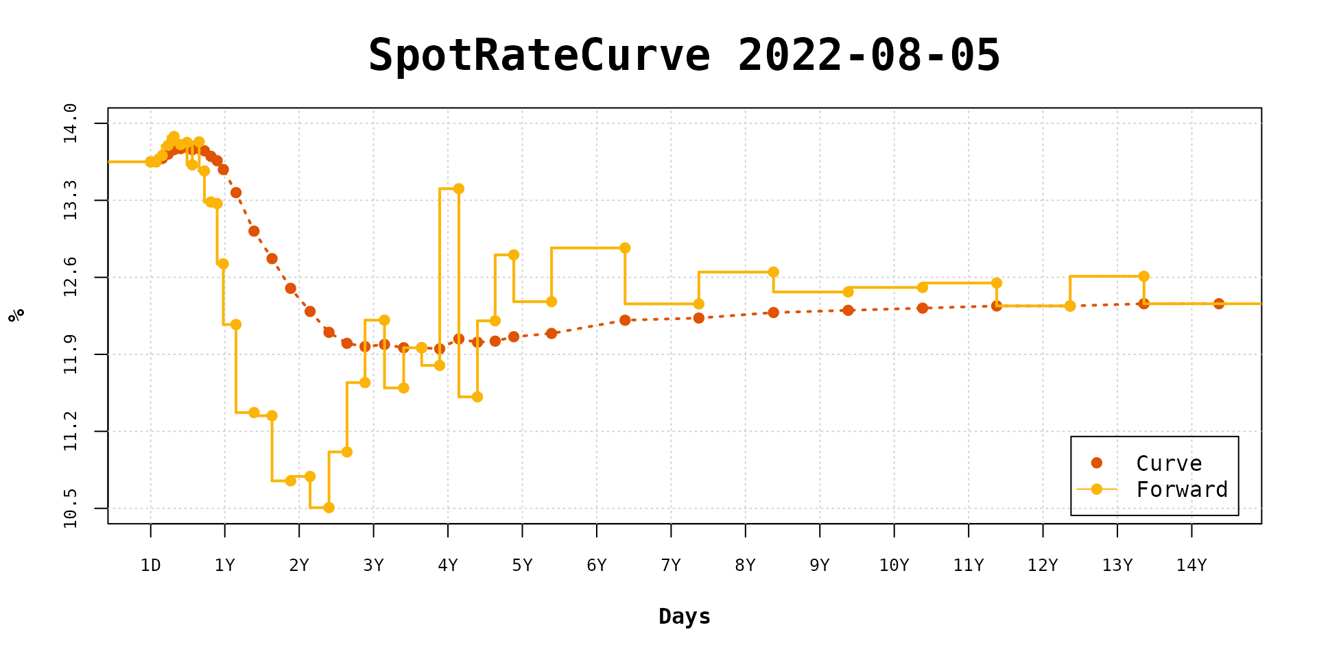
Forward rates with and without interpolation set

Once the interpolation is set, the plot method uses it to calculate daily forward rates. Otherwise, it uses the forward rates between the curve terms. Set the show_forward argument to TRUE to show the forward rates.

interpolation(sp_curve) <- NULL
plot(sp_curve, show_forward = TRUE, legend_location = "bottomright")

The forward rates are drawn with step lines.

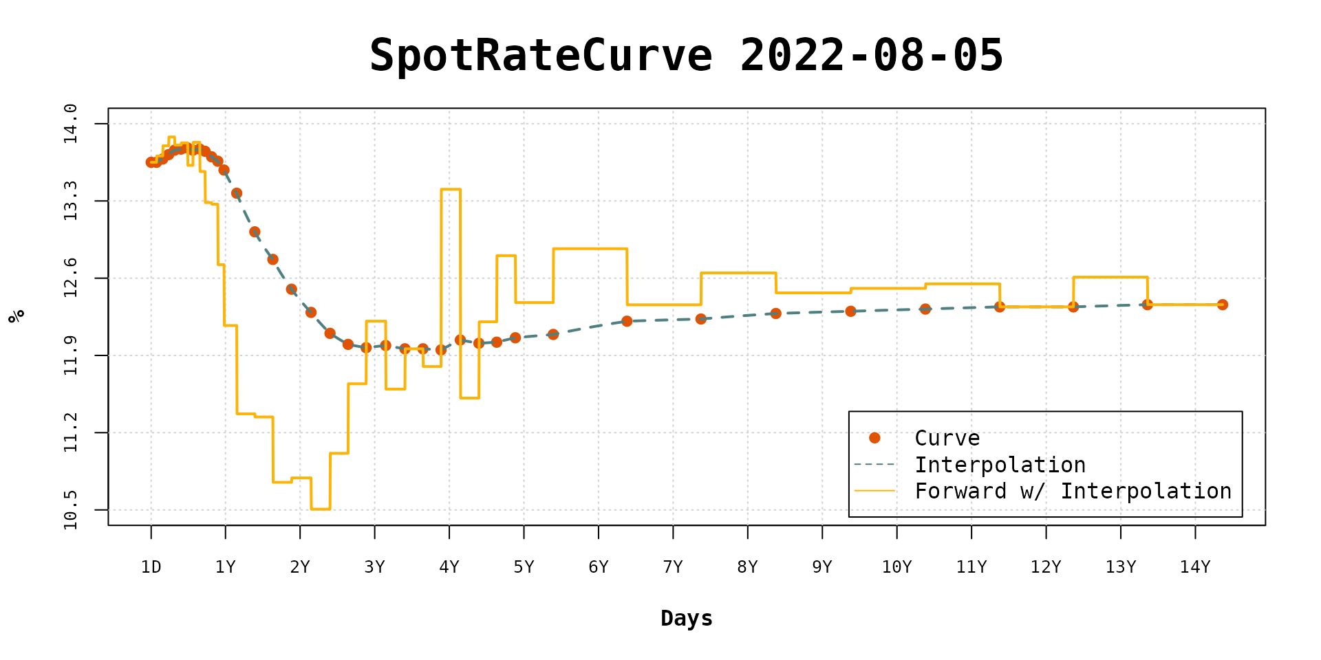
If the use_interpolation argument is TRUE then the daily forward rates are calculated with the defined interpolation.

interpolation(sp_curve) <- interp_flatforward()
plot(sp_curve, use_interpolation = TRUE, show_forward = TRUE, legend_location = "bottomright")

It is possible to note that the flat forward daily rates are fairly close to curve terms forward rates.

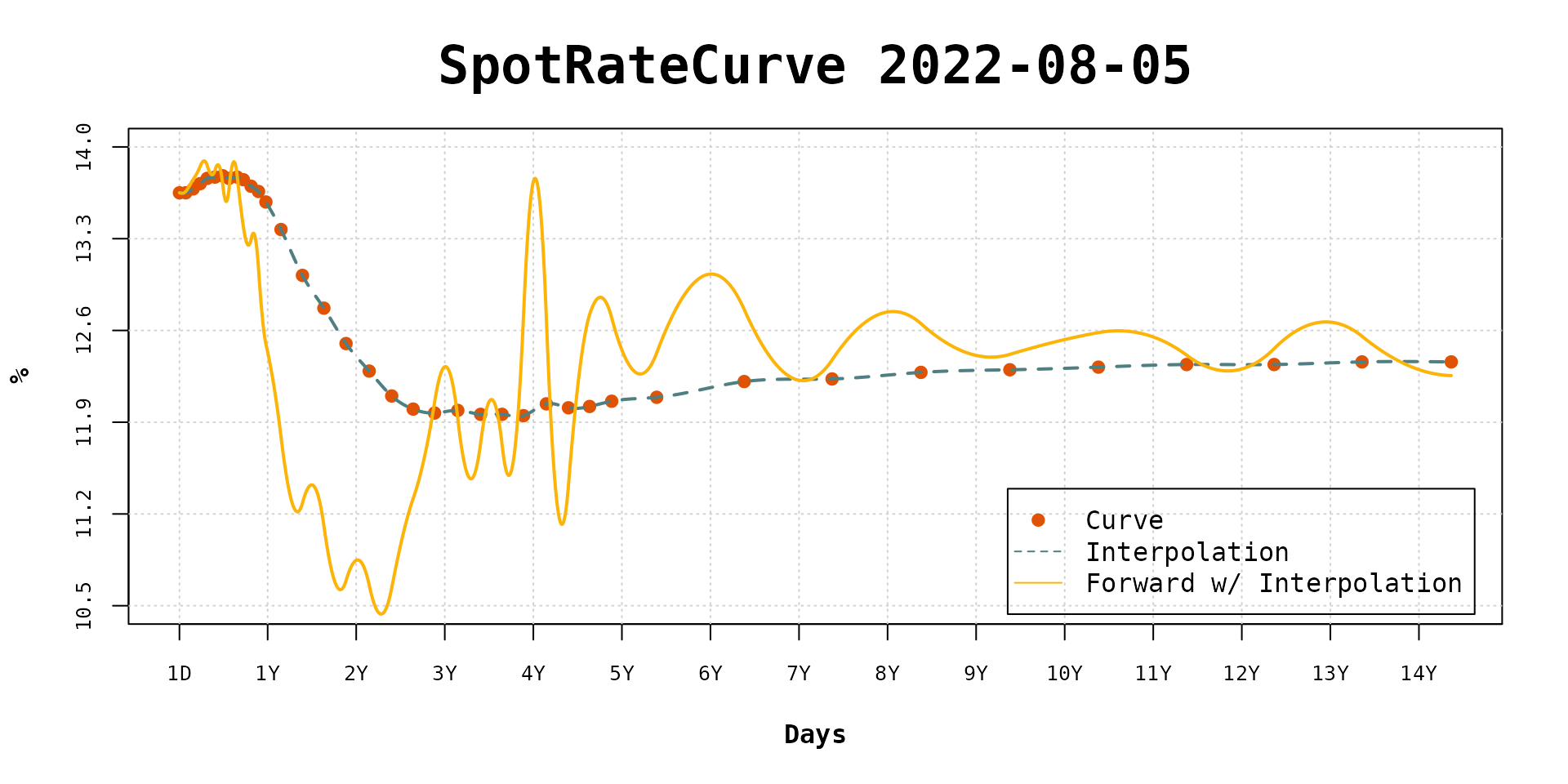
As the interpolation changes its effects can be viewed in the forward rates dynamic.

interpolation(sp_curve) <- interp_naturalspline()
plot(sp_curve, use_interpolation = TRUE, show_forward = TRUE, legend_location = "bottomright")

Interpolate with [[

Unset interpolation

Plot with interpolation

Forward rates with and without interpolation set

Interpolate with `[[`