Introduction to copom package
copom.RmdCreate a curve
Let’s create by hand the curve to be used in this tutorial. You must provide the curve terms and corresponding rates. The terms must be provided according to daycount used.
terms <- c(1, 3, 25, 44, 66, 87, 108, 131, 152, 172, 192, 214, 236, 277)
rates <- c(
  0.1065, 0.1064, 0.111, 0.1138, 0.1168, 0.1189, 0.1207, 0.1219,
  0.1227, 0.1235, 0.1234, 0.1236, 0.1235, 0.1235
)
curve <- spotratecurve(
  rates, terms, "discrete", "business/252", "Brazil/ANBIMA",
  refdate = as.Date("2022-02-23")
)
Here we use the daycount business/252, so the terms are business days.
Create the copom interpolation
Now we have a curve, we define the interpolation method by creating an Interpolation object with the function interp_flatforwardcopom. We pass a vector with the dates of the meetings to be used in the interpolation and set conflicts = "second". There are periods between meetings that have two points and, in this cases, the second point will be used in the interpolation.
Once the Interpolation object is created, it is set to the curve with the interpolation<- method.
copom_dates <- as.Date(
  c("2022-03-17", "2022-05-05", "2022-06-17", "2022-08-04")
)
interpolation(curve) <- interp_flatforwardcopom(copom_dates, "second")
Visualize the interpolation
With everything set the curve can be easily viewed with plot.
plot(curve,
  use_interpolation = TRUE, show_forward = TRUE,
  legend_location = "bottomright"
)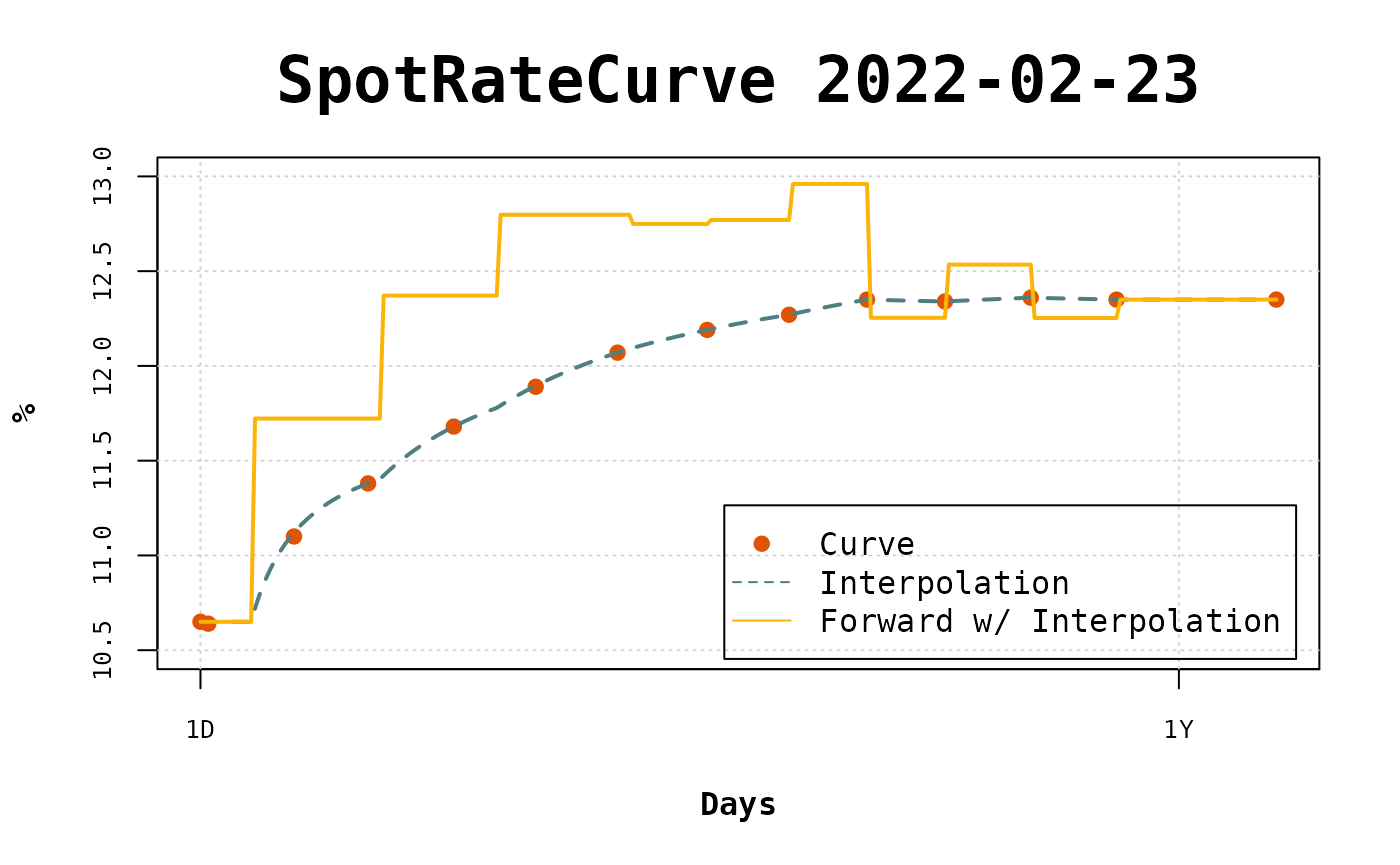
To compare with the flat forward interpolation let’s visualize the curve with this different intepolation.
interpolation(curve) <- interp_flatforward()
plot(curve,
  use_interpolation = TRUE, show_forward = TRUE,
  legend_location = "bottomright"
)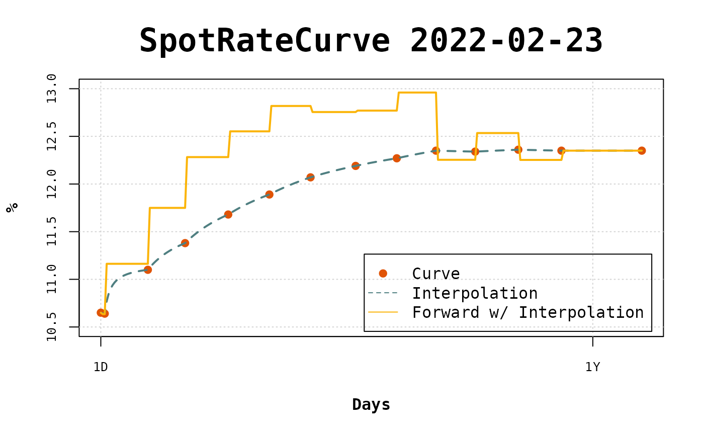
In the long term there isn’t mush difference, but in the short term the interpolated points and the forward rates are fairly different.