# A tibble: 1,105 × 6
   refdate    cur_days biz_days forward_date  r_252  r_360
   <date>        <int>    <dbl> <date>        <dbl>  <dbl>
 1 2020-03-19        1        1 2020-03-20   0.0365 0
 2 2020-03-19        4        2 2020-03-23   0.0365 0.0259
 3 2020-03-19        7        5 2020-03-26   0.0365 0.0372
 4 2020-03-19       11        7 2020-03-30   0.0365 0.0331
 5 2020-03-19       12        8 2020-03-31   0.0365 0.0347
 6 2020-03-19       13        9 2020-04-01   0.0365 0.036
 7 2020-03-19       14       10 2020-04-02   0.0365 0.0372
 8 2020-03-19       21       15 2020-04-09   0.0365 0.0372
 9 2020-03-19       27       18 2020-04-15   0.0365 0.0347
10 2020-03-19       32       21 2020-04-20   0.0365 0.0342
# ℹ 1,095 more rowsrb3
Curvas de juros nominais (prefixados)
Code
library(tidyverse)

ggplot(
  df_yc,
  aes(x = forward_date, y = r_252, group = refdate, color = factor(refdate))
) +
  geom_line(linewidth = 1) +
  labs(
    title = "Yield Curves for Brazil",
    subtitle = "Built using interest rates future contracts",
    caption = str_glue("Data imported using rb3 at {Sys.Date()}"),
    x = "Forward Date",
    y = "Annual Interest Rate",
    color = "Reference Date"
  ) +
  theme_light() +
  scale_y_continuous(labels = scales::percent)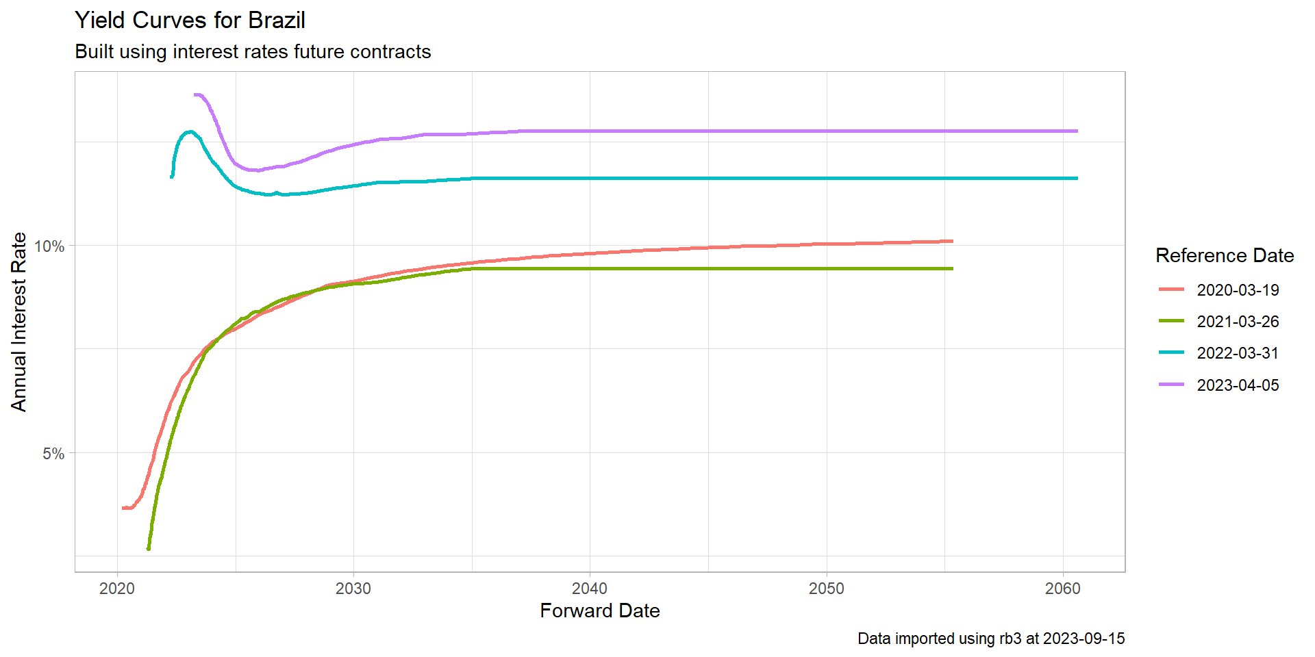
Curva de juros reais (cupom de IPCA)
Code
df_ipca_yc <- yc_ipca_mget(
  first_date = Sys.Date() - 255 * 5,
  last_date = Sys.Date(),
  by = 255
)

ggplot(
  df_ipca_yc,
  aes(x = forward_date, y = r_252, group = refdate, color = factor(refdate))
) +
  geom_line(linewidth = 1) +
  labs(
    title = "DIxIPCA Yield Curves for Brazil",
    subtitle = "Built using interest rates future contracts",
    caption = str_glue("Data imported using rb3 at {Sys.Date()}"),
    x = "Forward Date",
    y = "Annual Interest Rate",
    color = "Reference Date"
  ) +
  theme_light() +
  scale_y_continuous(labels = scales::percent)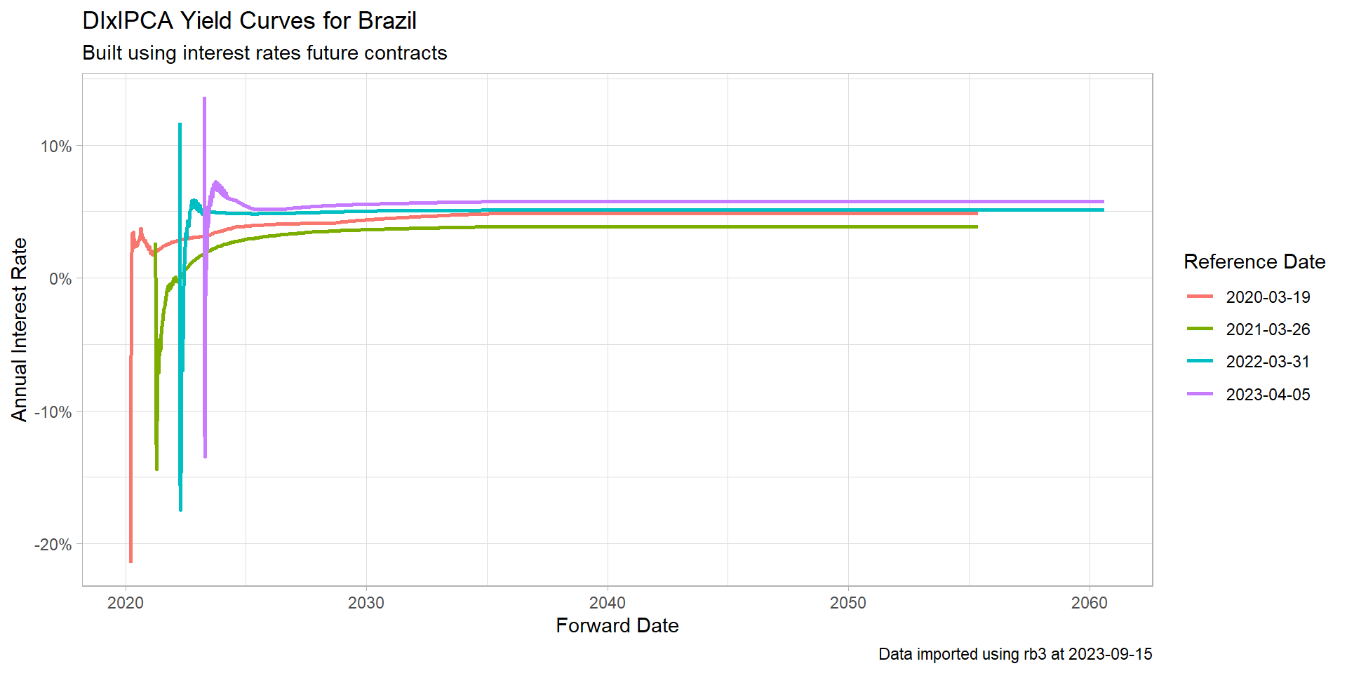
Inflação Implícita
Code
ggplot(
  inflation |> filter(forward_date < as.Date("2034-01-01")),
  aes(
    x = forward_date,
    y = inflation,
    group = refdate,
    color = factor(refdate)
  )
) +
  geom_line(linewidth = 1) +
  labs(
    title = "Implied Inflation for Brazil",
    subtitle = "Built using interest rates future contracts",
    caption = str_glue("Data imported using rb3 at {Sys.Date()}"),
    x = "Forward Date",
    y = "Annual Interest Rate",
    color = "Reference Date"
  ) +
  theme_light() +
  scale_y_continuous(labels = scales::percent)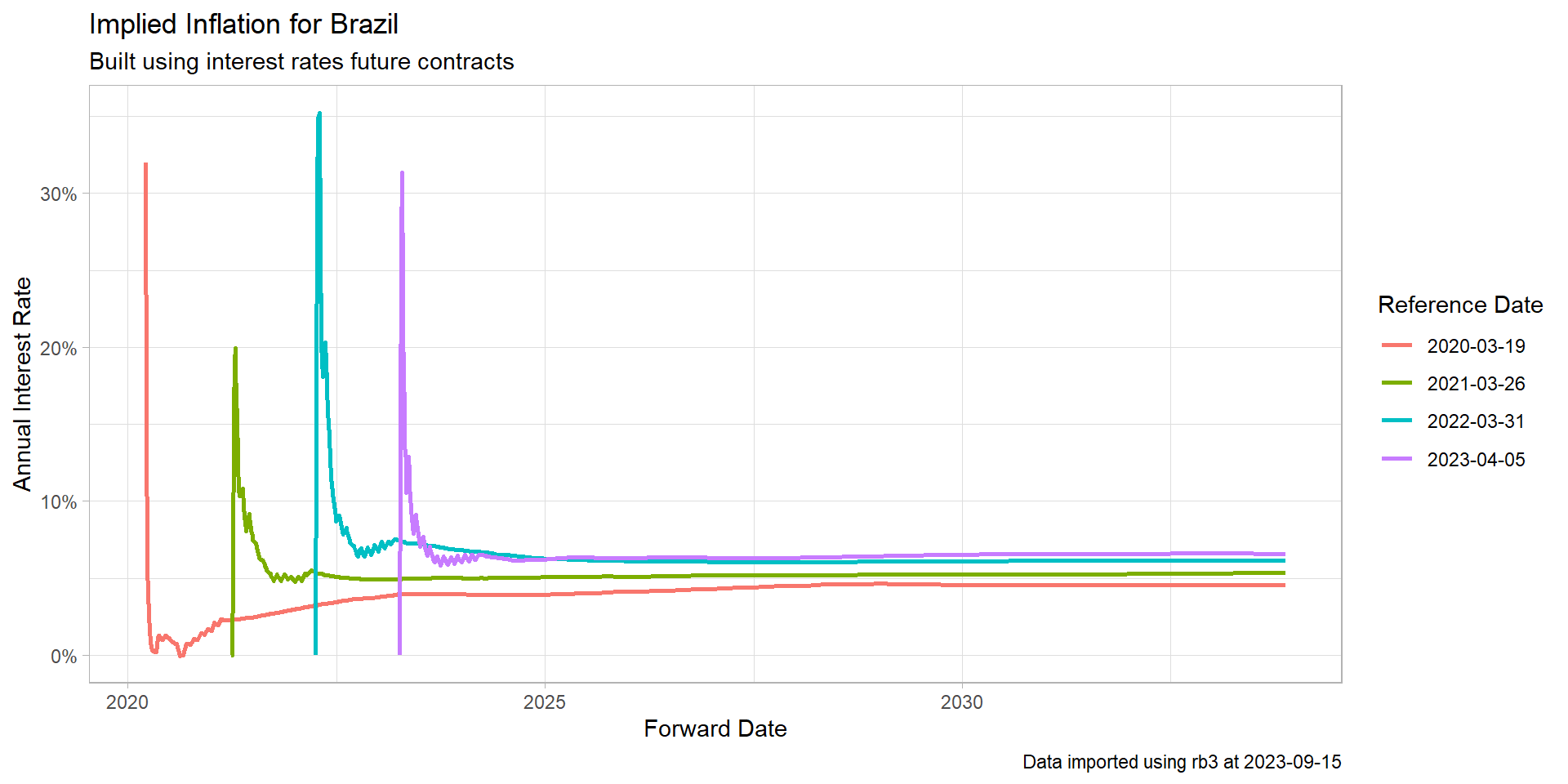
Curva de juros prefixados
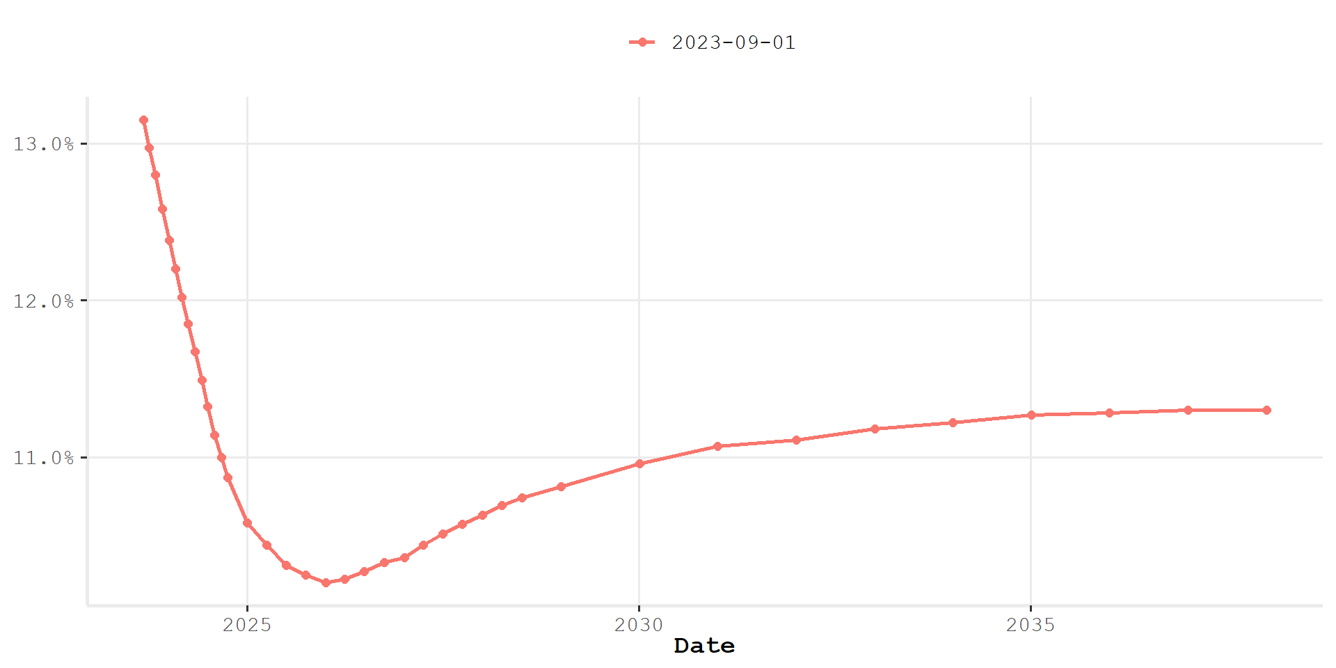
Histórico de juros prefixados de longo prazo
curves |>
    map_dfr(\(x) tibble(
        refdate = x@refdate,
        r_BRL_10y = as.numeric(x[[2520]])
    )) -> rates_10y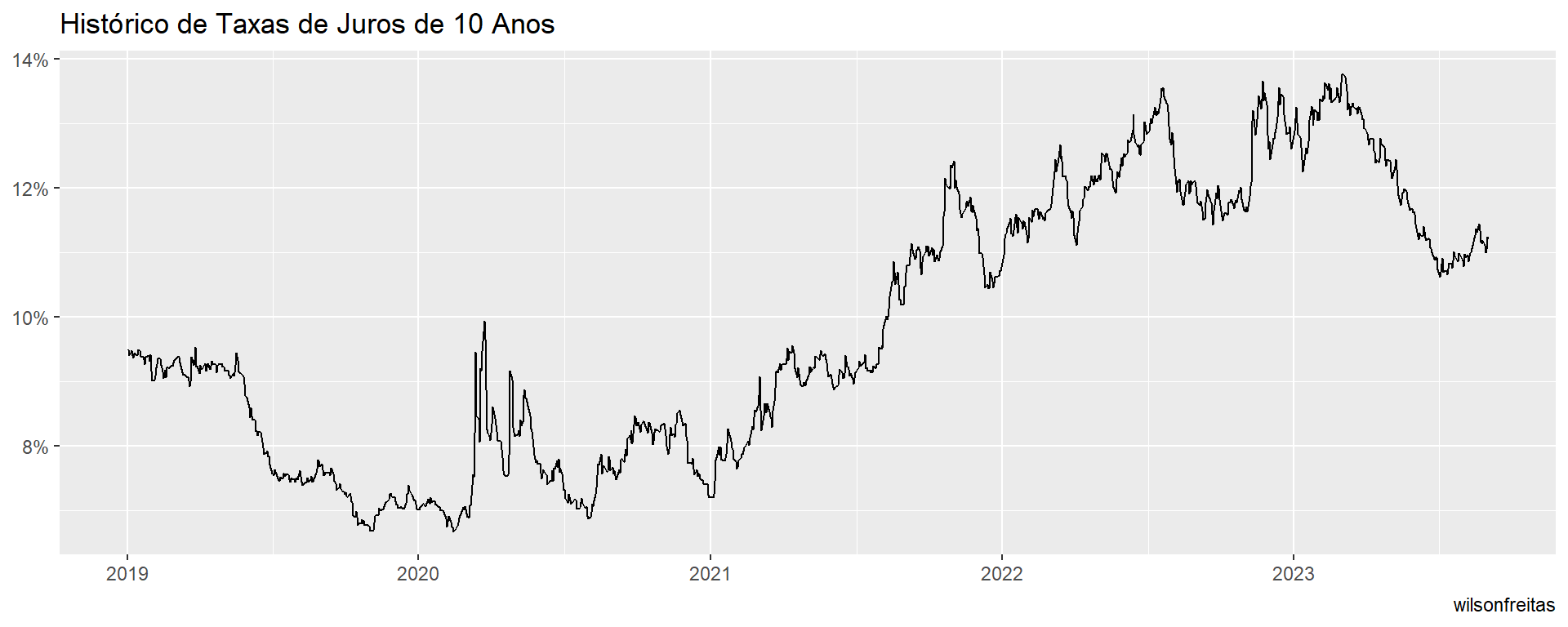
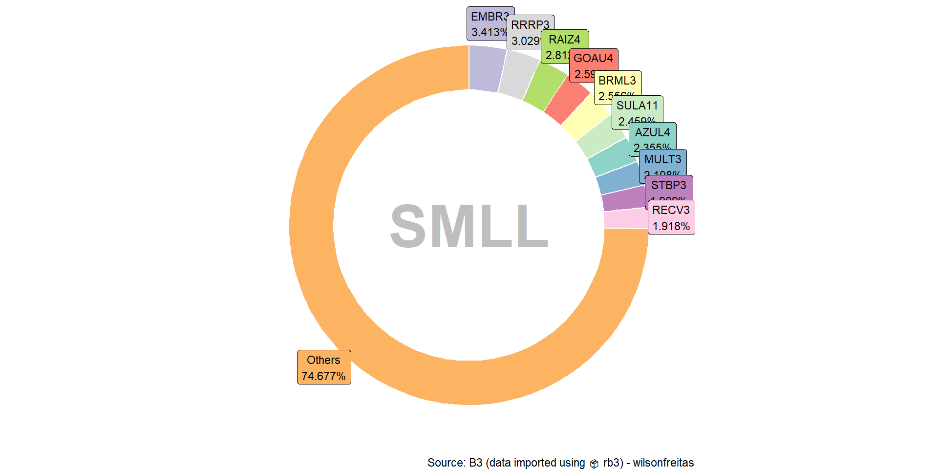
Composição de índices da B3
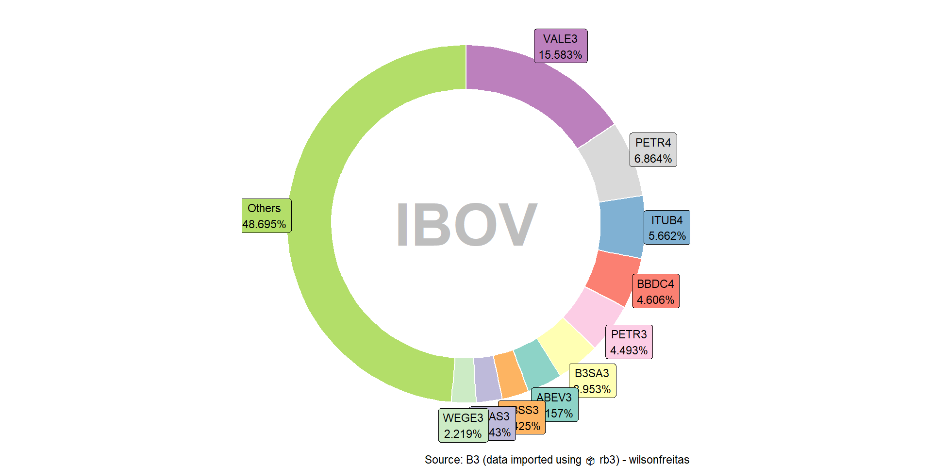
Composição de índices da B3
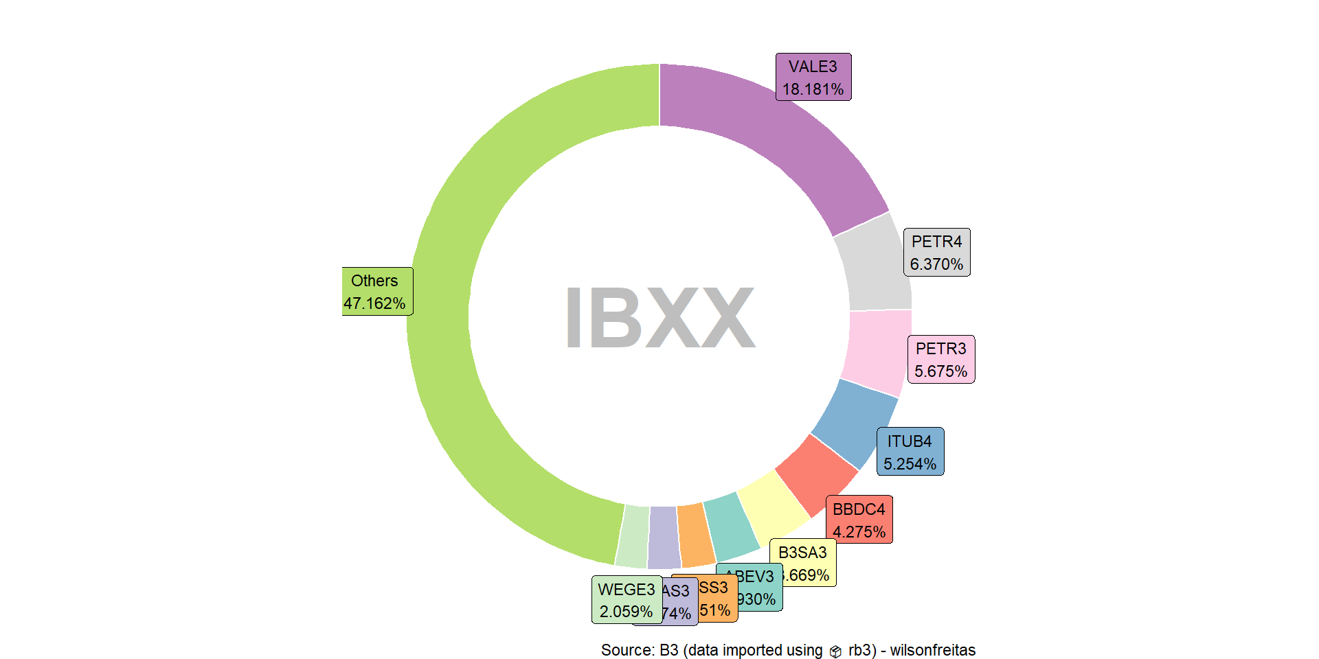
Composição de índices da B3
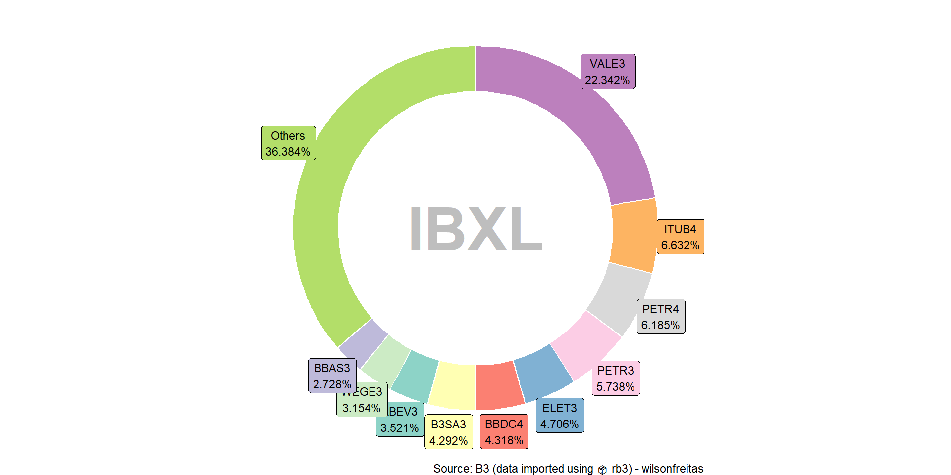
Composição de índices da B3
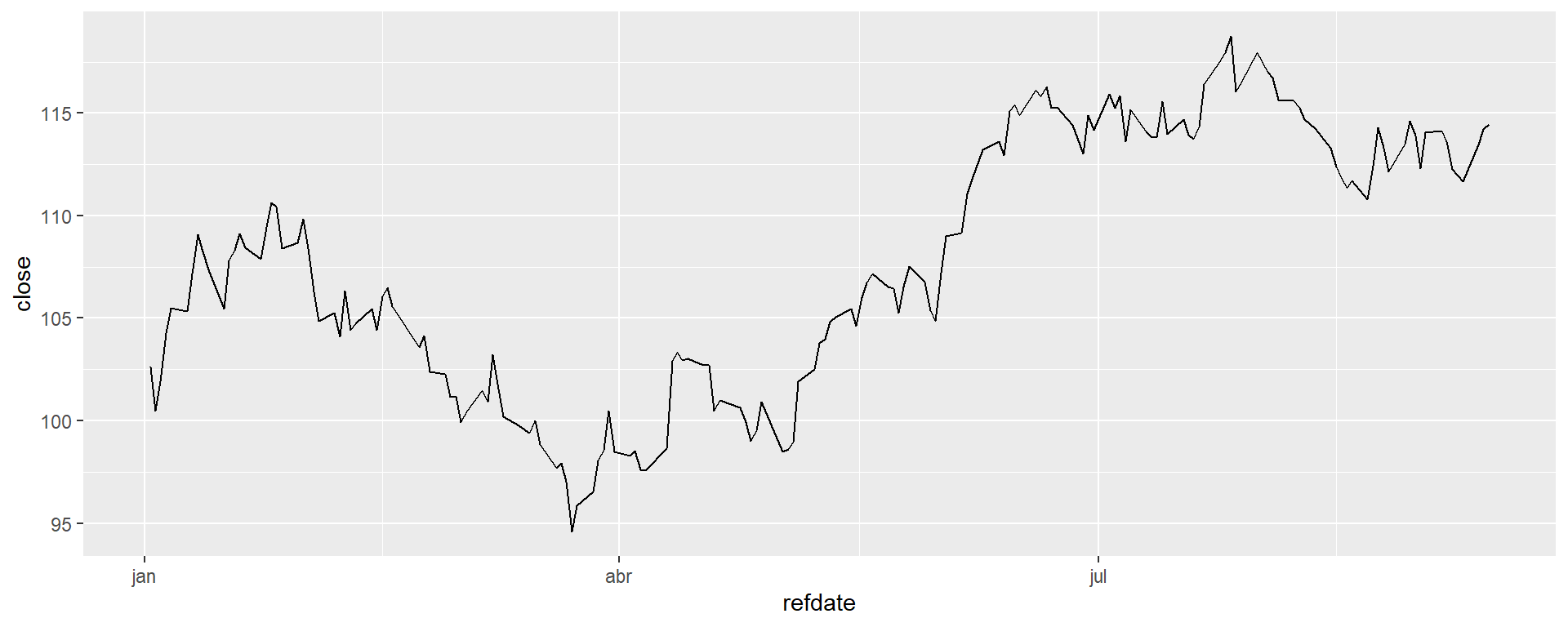
Série histórica de ETFs
Volatilidade implícita

Dinâmica da Volatilidade implícita
