SGS
A função bcb.sgs.get() obtém os dados do webservice do Banco Central,
interface JSON do serviço BCData/SGS -
Sistema Gerenciador de Séries Temporais (SGS).
Os parâmetros start e end aceitam strings YYYY-MM-DD, datetime.date, datetime.datetime ou bcb.utils.Date. Também é possível usar last para buscar os últimos n pontos disponíveis.
Timeout em consultas longas
Por padrão, as requisições usam o timeout global do cliente HTTP compartilhado.
Para consultas SGS com janelas grandes ou respostas lentas, informe timeout
na chamada. O valor é aplicado por tentativa HTTP; quando houver retry, cada
tentativa usa o mesmo timeout.
from bcb import sgs

df = sgs.get(11, start="1990-01-01", end="2026-01-01", timeout=120)
raw = sgs.get_json(11, start="1990-01-01", timeout=120)
Se a consulta continuar lenta mesmo com timeout maior, divida o período em janelas menores e concatene os resultados.
Formato tidy no SGS
Por padrão, bcb.sgs.get() retorna um DataFrame no formato largo. Para
retornar uma tabela longa, use tidy=True. Nesse modo, o DataFrame tem as
colunas Date, series e value. A coluna series usa o nome
informado em codes; quando nenhum nome é informado, usa o código numérico
da série.
In [1]: from bcb import sgs

In [2]: sgs.get({'SELIC': 11, 'IPCA': 433}, start='2024-01-01', tidy=True).head()
Out[2]:
        Date series     value
0 2024-01-01  SELIC       NaN
1 2024-01-02  SELIC  0.043739
2 2024-01-03  SELIC  0.043739
3 2024-01-04  SELIC  0.043739
4 2024-01-05  SELIC  0.043739
O parâmetro tidy só afeta o retorno output='dataframe'. Quando
output='text' é usado, a função continua retornando o JSON bruto.
Exemplos
In [3]: from bcb import sgs
In [4]: import matplotlib.pyplot as plt
In [5]: import matplotlib as mpl
In [6]: mpl.style.use('bmh')
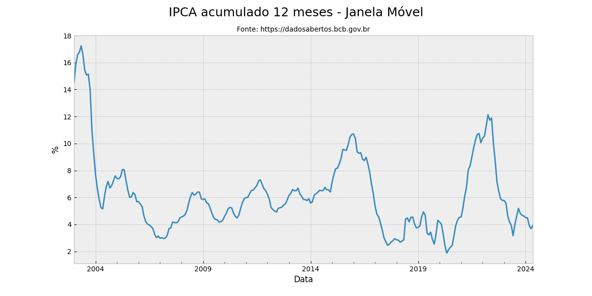
In [7]: df = sgs.get({'IPCA': 433}, start='2002-02-01')
In [8]: df.index = df.index.to_period('M')
In [9]: df.head()
Out[9]:
IPCA
Date
2002-02 0.36
2002-03 0.60
2002-04 0.80
2002-05 0.21
2002-06 0.42
In [10]: dfr = df.rolling(12)

In [11]: i12 = dfr.apply(lambda x: (1 + x/100).prod() - 1).dropna() * 100

In [12]: i12.head()
Out[12]:
              IPCA
Date
2003-01  14.467041
2003-02  15.847124
2003-03  16.572608
2003-04  16.769209
2003-05  17.235307
In [13]: i12.plot(figsize=(12,6))
Out[13]: <Axes: xlabel='Date'>

In [14]: plt.title('Fonte: https://dadosabertos.bcb.gov.br', fontsize=10)
Out[14]: Text(0.5, 1.0, 'Fonte: https://dadosabertos.bcb.gov.br')

In [15]: plt.suptitle('IPCA acumulado 12 meses - Janela Móvel', fontsize=18)
Out[15]: Text(0.5, 0.98, 'IPCA acumulado 12 meses - Janela Móvel')

In [16]: plt.xlabel('Data')
Out[16]: Text(0.5, 0, 'Data')

In [17]: plt.ylabel('%')
Out[17]: Text(0, 0.5, '%')

In [18]: plt.legend().set_visible(False)
Obtendo o JSON bruto
A função bcb.sgs.get_json() retorna o JSON bruto da API para um único código.
Para pipelines de dados onde o dado bruto deve ser persistido antes de qualquer transformação,
o parâmetro output='text' pode ser passado à função bcb.sgs.get().
Para um único código é retornada uma str; para múltiplos códigos é retornado um dict
mapeando código inteiro → JSON string.
from bcb import sgs

# único código → str
raw = sgs.get(433, start='2024-01-01', output='text')

# múltiplos códigos → dict[int, str]
raws = sgs.get([433, 189], start='2024-01-01', output='text')
# raws[433] → JSON string do IPCA
# raws[189] → JSON string do IGP-M

# salvar em disco
with open('ipca_raw.json', 'w') as f:
    f.write(raw)
O JSON retornado é um array de objetos com os campos data e valor, exatamente como
devolvido pela API BCData/SGS.
O comportamento padrão (retorno de DataFrame) é mantido quando o parâmetro não é informado.
Dados de Inadimplência de Operações de Crédito
Os modos aceitos são PF (pessoas físicas), PJ (pessoas jurídicas) e total; all é aceito como alias de total. Os locais devem ser todos estados ou todos regiões, sem misturar os dois tipos na mesma chamada.
In [19]: from bcb.sgs.regional_economy import get_non_performing_loans

In [20]: from bcb.utils import BRAZILIAN_REGIONS, BRAZILIAN_STATES

In [21]: import pandas as pd

In [22]: get_non_performing_loans(["RR"], last=10, mode="all")
Out[22]:
              RR
Date
2025-07-01  5.06
2025-08-01  5.21
2025-09-01  5.02
2025-10-01  5.24
2025-11-01  5.24
2025-12-01  5.17
2026-01-01  5.42
2026-02-01  5.64
2026-03-01  5.49
2026-04-01  5.96
In [23]: northeast_states = BRAZILIAN_REGIONS["NE"]

In [24]: get_non_performing_loans(northeast_states, last=5, mode="pj")
Out[24]:
              AL    BA    CE    MA    PB    PE    PI    RN    SE
Date
2025-12-01  2.65  2.94  3.47  5.83  8.31  2.96  2.11  3.82  4.22
2026-01-01  3.14  3.18  3.70  6.12  8.61  3.22  2.12  3.77  4.55
2026-02-01  3.36  4.22  3.81  6.23  8.76  3.35  2.33  3.98  4.76
2026-03-01  3.46  3.17  3.64  6.16  8.67  3.30  2.38  3.79  4.64
2026-04-01  3.46  3.67  3.71  6.56  8.96  3.52  2.56  3.91  4.68
In [25]: get_non_performing_loans(BRAZILIAN_STATES, mode="PF", start="2024-01-01")
Out[25]:
              AC    AP    AM    PA    RO  ...    RJ    SP    PR    RS    SC
Date                                      ...
2024-01-01  3.49  4.09  5.40  4.16  2.76  ...  5.33  3.45  2.76  2.48  2.85
2024-02-01  3.48  4.05  5.25  4.15  2.78  ...  5.25  3.43  2.75  2.51  2.84
2024-03-01  3.43  4.01  5.18  4.09  2.81  ...  5.17  3.36  2.74  2.53  2.81
2024-04-01  3.46  4.10  5.15  4.09  2.85  ...  5.13  3.41  2.75  2.53  2.81
2024-05-01  3.54  4.22  5.26  4.15  2.99  ...  5.14  3.46  2.83  2.60  2.87
2024-06-01  3.50  4.11  5.14  4.09  3.07  ...  5.04  3.40  2.76  2.61  2.79
2024-07-01  3.49  4.13  5.14  4.14  3.16  ...  5.02  3.43  2.87  2.61  2.82
2024-08-01  3.41  4.03  5.05  4.13  3.23  ...  4.97  3.42  3.02  2.58  2.81
2024-09-01  3.55  4.06  4.99  4.16  3.24  ...  4.90  3.39  3.01  2.54  2.79
2024-10-01  3.55  3.98  4.86  4.21  3.26  ...  4.84  3.35  2.97  2.49  2.74
2024-11-01  3.49  3.95  4.74  4.23  3.30  ...  4.80  3.32  2.94  2.41  2.70
2024-12-01  3.52  4.02  4.64  4.20  3.34  ...  4.70  3.28  2.87  2.29  2.66
2025-01-01  3.86  4.42  4.91  4.48  3.67  ...  5.08  3.56  3.11  2.51  2.87
2025-02-01  3.95  4.50  5.04  4.61  3.85  ...  5.13  3.64  3.22  2.73  2.99
2025-03-01  3.84  4.57  4.91  4.60  3.86  ...  5.10  3.64  3.22  2.90  3.03
2025-04-01  4.08  4.90  5.17  4.82  4.18  ...  5.30  3.80  3.47  3.18  3.26
2025-05-01  4.19  5.03  5.35  4.96  4.27  ...  5.46  3.90  3.54  3.37  3.39
2025-06-01  4.30  5.19  5.44  5.03  4.23  ...  5.45  3.91  3.51  3.44  3.43
2025-07-01  4.51  5.34  5.69  5.27  4.65  ...  5.59  4.06  3.76  3.66  3.59
2025-08-01  4.73  5.39  5.82  5.45  4.99  ...  5.67  4.19  4.08  3.94  3.72
2025-09-01  4.63  5.34  5.82  5.46  5.08  ...  5.62  4.13  4.05  4.15  3.61
2025-10-01  4.90  5.53  5.94  5.84  5.47  ...  5.75  4.24  4.18  4.58  3.73
2025-11-01  4.96  5.51  5.95  5.90  5.75  ...  5.74  4.26  4.29  4.68  3.77
2025-12-01  5.20  5.64  6.06  5.92  5.70  ...  5.71  4.21  4.17  4.67  3.76
2026-01-01  5.56  5.92  6.34  6.26  6.09  ...  5.99  4.50  4.52  5.00  4.01
2026-02-01  5.66  6.63  6.71  6.44  6.40  ...  6.36  4.73  4.74  5.33  4.17
2026-03-01  5.82  6.64  6.68  6.44  6.32  ...  6.23  4.63  4.62  5.26  4.07
2026-04-01  6.37  6.70  6.78  6.76  6.52  ...  6.38  4.78  4.82  5.40  4.21

[28 rows x 27 columns]