The so famous EWMA (Exponentially Weighted Moving Average) model
$$ \hat\sigma^2_t = \lambda\hat\sigma^2_{t-1} + (1 - \lambda)r^2_t $$
used to estimate the volatility of asset returns. It is extensively used in Risk Management and is in the core of RiskMetrics. EWMA has a magic parameter $\lambda$ that is $0.94$ in the absolutely great amount of Risk Management Systems running World Wide. I can't tell if it is JPMorgan's fault or it's one more of those situations where the idiots are taking over, but why $0.94$, why people seem to accept it without have any idea where it came from. (Why so serious.) But ok, JPM said that and JPM is great, so I see no reason to question that. However, there is another point which disturbs me more, the well accepted EWMA's period of convergence.
It is well known, among risk management practioneers, that EWMA with $\lambda=0.94$ has a period of convergence that is about 60 time steps. Unfortunately, for some series, you don't have 60 points of historical data and EWMA can't reach its convergence.
Oh! It looks a bad thing
Some practioneers usually use a proxy to fulfill that pre-requisite and that proxy can be any related asset (yeah! a bit heuristic). Of course I have one question: does it really matters?. I mean, is it really necessary to use a proxy to have a good estimative of the volatility? Use no proxy isn't an option? Or it is operational pre-requisite, the risk management system can't compute the volatility of a time series that doesn't enough historical data to guarantee the convergence its convergence.
I am going too far and I am afraid my anger on that subject attracts more attention than what really matters: how many returns are necessary to estimate $\hat\sigma^2_t$?
I don't know the answer and I do think it has no right answer. I did an experiment in order to try to observe the EWMA's convergence and the results gave me a little hope.
Bootstraping time series
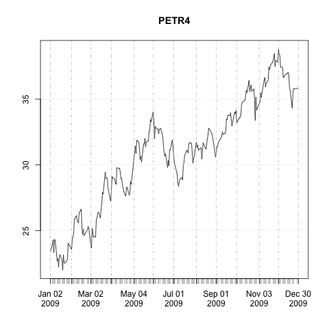
I picked up PETR4 time series and computed the returns for the year of 2009.
library(xts)
table.df <- read.csv("PETR4.daily.raw.csv", header=TRUE, stringsAsFactors=TRUE)
rownames(table.df) <- as.Date(table.df[, "Date"])
prices.df <- table.df[, "Adj.Close", drop=FALSE]
prices.x <- as.xts(prices.df[,1], order.by=as.Date(rownames(prices.df)))
ret.x <- diff(log(prices.x))['2009']
plot(prices.x['2009'])
boxplot(coredata(ret.x))
The graph below shows time series of prices of PETR4 for the year of 2009—that seemed to be a good year for PETR4.
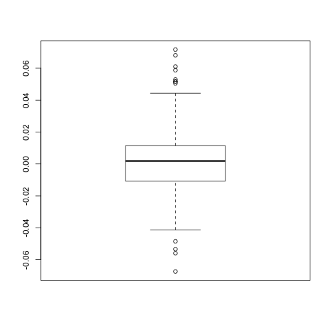
To have an idea of how volatile its was in that year I looked at the box plot of returns.
I put the returns into a matrix because it is easier to work with this structure instead of working with a time series.
rets <- coredata(first(ret.x, n=100))
Now, assuming that the returns are IID I ran a bootstrap computating EWMA for each sample of the time series generated by boot.
library(boot)
ewma.boot = function(r, idx) {
    sig.p <- 0
    sig.s <- vapply(idx, function(i) sig.p <<- sig.p*lambda + (r[i]^2)*(1 - lambda), 0)
    return(sqrt(sig.s))
}
lambda <- 0.94
r.ewma.boot <- boot(rets, statistic=ewma.boot, R=200)
In the end of the bootstrap process I got a sample of EWMA time series in the variable r.ewma.boot.
r.ewma.boot is an instance of the class boot, which is returned by the function with the same name.
It has an attribute t which stores all samples generated by the execution of boot and other attribute t0 which stores the result for the original time series.
I ran that experiment with $\lambda=0.94$, but it can be run with any other value.
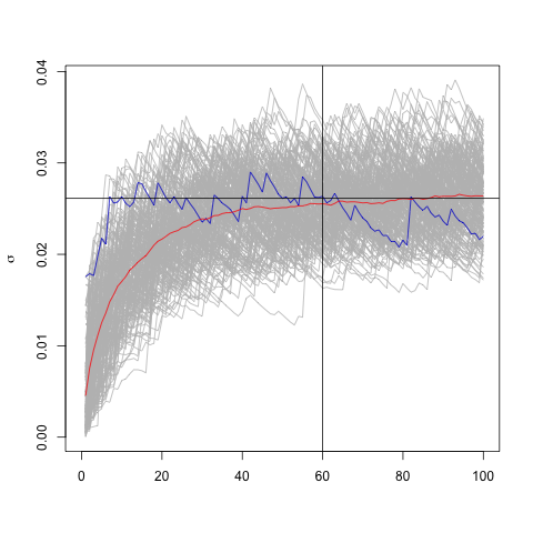
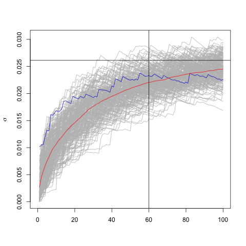
The red line is the mean volatility and as we can observe, it converges to the long run standard deviation—shown by the black horizontal line. And, as some practioneers usually say, 60 time steps isn't a bad choice for EWMA's convergence, when $\lambda=0.94$. For $\lambda=0.98$ we need more time steps to reach the convergence—as can be seen in the image below the time series used has 200 time steps instead of 100.
We clearly observe the convergence, I tend to believe it is in distribution.
Assintoticaly the mean value of EWMA estimator converges to the sample sd, but EWMA gives a local estimative of volatility as we observe in the blue line.
Simulated time series
I extended that experiment for an environment where I could control all variables. So, following the assumption of IID returns I created one sample of returns and bootstraped it.
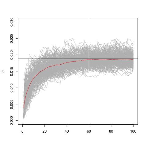
We observe the convergence to the sample sd which differs a little from the theoretical standard deviation (0.02).
As expected the convergence with $\lambda=0.94$ occurs within the same numbers of time steps we've observed in the real time series.
This result might help confirming the assumption that assets' returns are IID.
lambda <- 0.94
sig.m <- matrix(0, nrow=200, ncol=100)
r <- 0.02*rnorm(dim(sig.m)[2])
plot(0, type="n", xlab='', ylab=expression(sigma),
    xlim=c(0,dim(sig.m)[2]), ylim=c(0,0.03))
for (k in 1:dim(sig.m)[1]) {
    sig.p <- 0
    sig.s <- vapply(sample(1:dim(sig.m)[2]), function(i) sig.p <<- sig.p*lambda + (r[i]^2)*(1 - lambda), 0)
    lines(sig.m[k, ] <- sqrt(sig.s), col="grey")
}
abline(h=sd(r), col="black")
abline(v=60, col="black")
lines(apply(sig.m, 2, mean), col="red")
Conclusion
I am obliged to agree that the market convention isn't silly. Indeed, 60 times steps are reasonable for $\lambda=0.94$ as more time steps are made necessary for greater values of $\lambda$. Though I couldn't validate the use of a proxy for series that don't have this minimal number of points I see that I can't use EWMA without it.